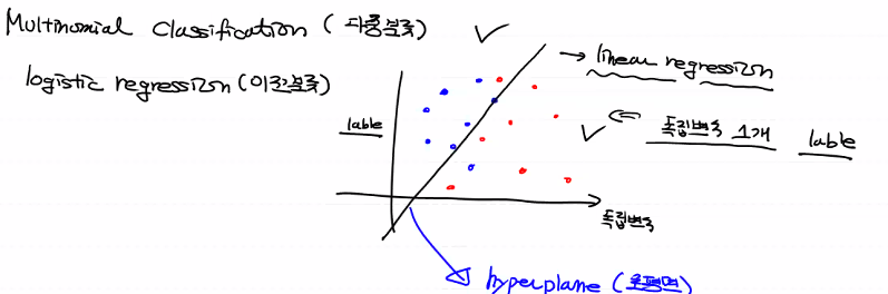
이진 분류에서 기준선을 초평면(hyperplane)이라고 불러요!
독립변수 개수에 따라 초평면의 형태가 변해요!.
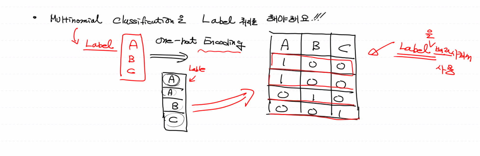
multinomial classification(다중 분류)
이진 분류하는 logistic을 여러 개 모아놓은 것.
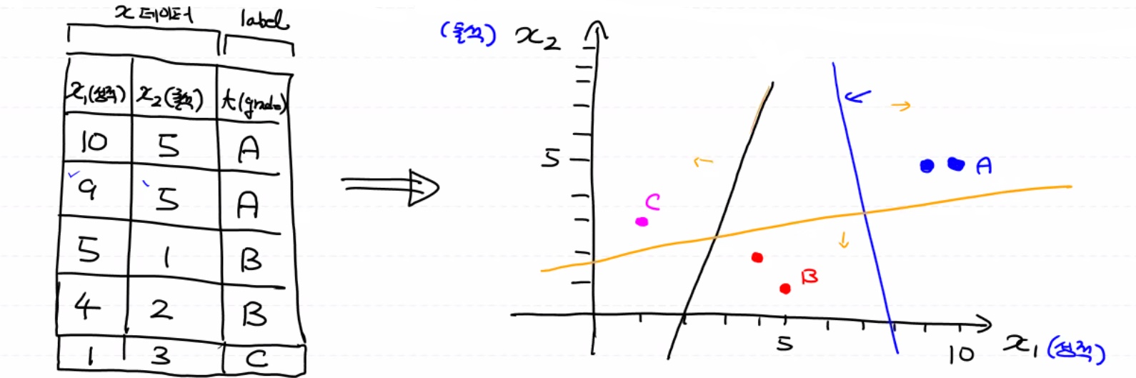
여러 개 중 하나씩 생각해요. 이것을 하나로 묶어 계산해요.
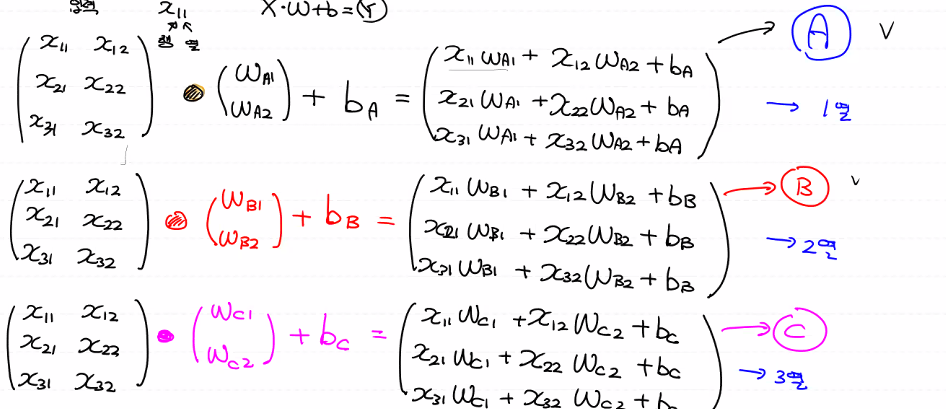
계산해보면, 2줄만 표현할게요...
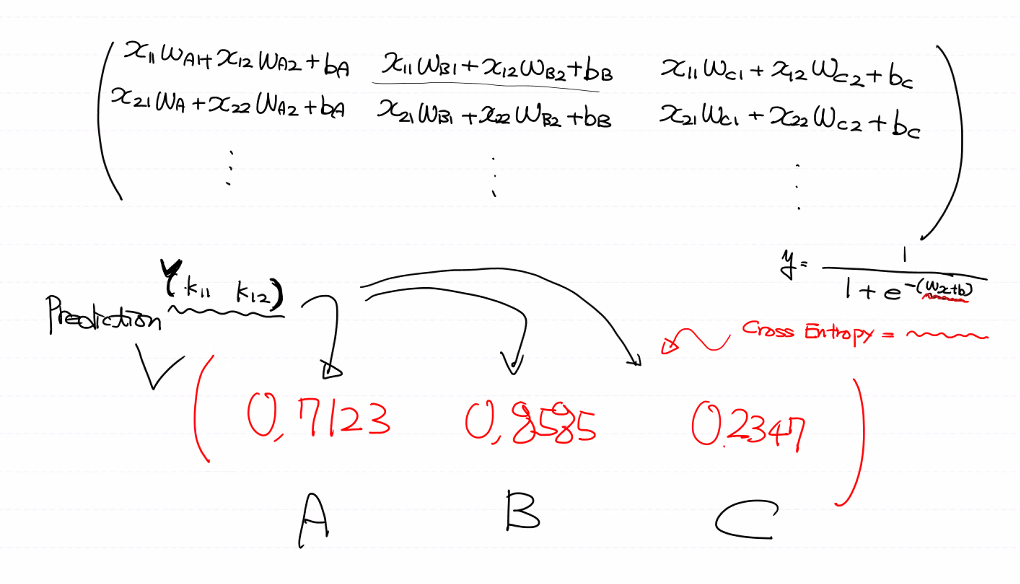
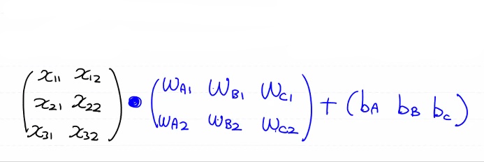
행렬식으로 한 번에 계산했어요!!
하지만 우리가 알고 싶은 것은 각각의 개별적인 확률이 아니라 A B C 중 A의 확률, A B C 중 B의 확률,
A B C 중 C의 제각각 확률이 알고 싶어요.
그래서 sigmoid모델과 Cross Entropy가 변해요. sigmoid 함수가 Softmax로 바뀌어요!!
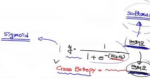
그러면 식이 이런 식으로 떨어져요.(전체에 대한 각각의 확률, 여러 개 중 하나가 될 확률)

기본 시작은 초평면 역할을 하는 Linear regression으로 시작해요.
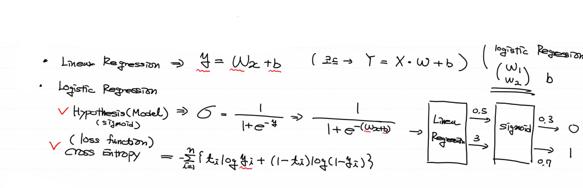
이진 분류는 w가 2개예요 multinomial로 넘어오면서 class의 개수에 따라 w와 bias가 늘었어요.(모양이 변함)
행의 개수는 독립변수의 수(column의 수)와 같아야 하고, 열의 개수는 class의 개수와 일치해야 해요. 바이어스(binary classification)의 수도 같이 늘어요!
여러 개 중의 확률을 구하기 때문에 합해서 나누는 거예요. 이진 분류는 w가 2개예요.
multinomial로 넘어오면서 class의 개수에 따라 w와 bias가 늘었어요.(모양이 변함)
행의 개수는 독립변수의 수(column의 수)와 같아야 하고, 열의 개수는 class의 개수와 일치해야 해요.
바이어스(binary classification)의 수도같이 늘어요!
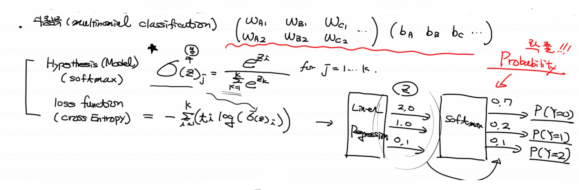
여러 개 중의 확률을 구하기 때문에 합해서 나누는 거예요.
multinomial classification(다중분류)는 반드시 Label 처리를 해야 해요!!
BMI 지수로 multinomial classification를 해보아요! label이 총 3개 0 thin, 1 normal, fat 2
# multinomial classification(다중 분류) - BMI
# Tensor flow로 구현해 보아요!
import numpy as np
import pandas as pd
from sklearn.model_selection import train_test_split
from sklearn.preprocessing import MinMaxScaler
from scipy import stats
import tensorflow as tf
# Raw data Loading
# skiprows 제일위에 label 3줄 빼고 읽어요!
df = pd.read_csv('./data/bmi/bmi.csv', sep=',', skiprows=3)
# 결측치 처리
# df.isnull().sum() # 결측치가 없네요!!
# 이상치 처리
# zscore_threshold=1.8
# df.loc[np.abs(stats.zscore(df['height'])) > zscore_threshold, :] # height에는 이상치가 없어요!
# df.loc[np.abs(stats.zscore(df['weight'])) > zscore_threshold, :] # weight에는 이상치가 없어요!
# train , validation data 분할
train_x_data, valid_x_data, train_t_data, valid_t_data = \
train_test_split(df[['height', 'weight']],
df[['label']],
test_size=0.3,
stratify=df[['label']],
random_state=1)
# Normalization(정규화) 처리
scaler = MinMaxScaler()
scaler.fit(train_x_data) # train_x_data를 scaler기준으로 삼아요
train_x_data_norm = scaler.transform(train_x_data)
valid_x_data_norm = scaler.transform(valid_x_data)
del train_x_data # 사용하지 않는 데이터는 삭제!
del valid_x_data
# ONE-HOT Encoding 처리(Label처리)
# 0 -> 1 0 0
# 1 -> 0 1 0
# 2 -> 0 0 1
# 3가지 방법 중 하나를 이용해서 One-Hot Encoding을 처리
# numpy가 가지는 방법을 이용, sklearn의 기능을 이용, Tensor flow의 기능을 이용
# 우리는 tensor flow 기능을 이용해서 one-hot encoding을 사용
# depth는 class의 개수를 알려줘요!!
sess = tf.Session()
train_t_data_onehot = sess.run(tf.one_hot(train_t_data, depth=3))
valid_t_data_onehot = sess.run(tf.one_hot(valid_t_data, depth=3))
del train_t_data # x 데이터는 정규화
del valid_t_data # t 데이터는 one hot
# 데이터 준비가 다 됐으니 Tensor flow graph를 그려보아요!
# placeholder
X = tf.placeholder(shape=[None,2], dtype=tf.float32) # 독립변수 키, 몸무게 2개
T = tf.placeholder(shape=[None,3], dtype=tf.float32) # class 개수 3개
# Weight & bias
W = tf.Variable(tf.random.normal([2,3]))
b = tf.Variable(tf.random.normal([3]))
# Hypothesis(Model) => multinomial classification
logit = tf.matmul(X,W) + b
H = tf.nn.softmax(logit) # H = tf.sigmoid(logit) => binary classification
# loss function
# binary classification loss
# loss = tf.reduce_mean(tf.nn.sigmoid_cross_entropy_with_logits(logits=logit,
# labels=T))
# multinolial classification loss
loss = tf.reduce_mean(tf.nn.softmax_cross_entropy_with_logits_v2(logits=logit,
labels=T))
# train
train = tf.train.GradientDescentOptimizer(learning_rate=1e-1).minimize(loss)
# 초기화
sess.run(tf.global_variables_initializer())
# 반복학습
for step in range(10000):
tmp, loss_val = sess.run([train, loss],
feed_dict={X:train_x_data_norm,
T:train_t_data_onehot.reshape(-1,3)})
if step % 1000 == 0:
print('loss : {}'.format(loss_val))
# loss : 0.24836672842502594
# Evaluation(모델 평가)
# binary classification과는 달라요!
# 입력 데이터 하나 넣었을 때 예를 들어
# X => [188 78] 정규화 처리해서 [0.7 0.2]
# H => [[0.6 0.3 0.1]] 0
# T => [1 0 0 ] 0
predict = tf.argmax(H,1)
correct = tf.equal(predict, tf.argmax(T,1))
acc = tf.reduce_mean(tf.cast(correct, dtype=tf.float32))
print('accuracy(정확도) : {}'.format(sess.run(acc, feed_dict={X:valid_x_data_norm,
T:valid_t_data_onehot.reshape(-1,3)})))
# accuracy(정확도) : 0.9823333621025085
# Prediction
predict_data = [[187, 78]]
predict_data_norm = scaler.transform(predict_data)
result = sess.run(predict, feed_dict={X:predict_data_norm})
print(result) # [1] => normal
'머신러닝 딥러닝' 카테고리의 다른 글
| 0909 Tensor flow 2.x, keras in tensor 2.x (0) | 2021.09.09 |
|---|---|
| 0909 multinomial classification - MNIST (0) | 2021.09.09 |
| 0908 확률적 경사 하강법(SGD classifier) (0) | 2021.09.08 |
| 0906 titanic (0) | 2021.09.06 |
| 0906 Logistic Regression (0) | 2021.09.06 |


댓글